Deploy a Custom YOLO Model on the Synaptics Torq NPU

Detecting objects in images or in a camera feed is a very common and useful vision-based use case of edge AI. A few examples include detecting hard hats for worksite safety and vehicles for traffic monitoring. Pretrained object detection models typically do not detect the objects that your application needs. So for a real product, developers need to retrain models. In this post, we walk through a practical workflow for retraining an object detection model and converting it to run on the Torq™ NPU in Astra SL2610-Series processors.

About YOLO and Ultralytics

YOLO ("You Only Look Once") is a popular family of object detection models. It detects objects in a single pass over the image, which makes it efficient enough to run in real time on many platforms. YOLO is a single-stage detector: one pass through a convolutional backbone, a multi-scale feature-pyramid neck, and a head that predicts boxes and classes on a grid. YOLOv8 Nano (YOLOv8n) is a stable, efficient, and widely deployed version of YOLO, which we are using in this example.

Ultralytics provides pretrained models and training tools to help developers retrain models to suit their needs. They maintain the ultralytics Python package, which bundles the YOLOv8 and later YOLO model families with a workflow for training, validation, prediction, and export. The models are PyTorch under the hood — a checkpoint is a standard .pt file — so you can fine-tune on a custom dataset and export to ONNX, TFLite, and other formats. As with any software or tool, make sure to review the Ultralytics licensing terms to ensure they are compatible with your project.

Training to Deployment Workflow

The validated flow to retrain and deploy a model is: YOLOv8 training -> Model Export & Preprocessing -> Quantization -> Conversion to TOSA -> Compilation.

The conversion steps shown here were validated with a 320 x 320 YOLOv8 object-detection model. Some details, particularly output normalization and tensor shapes, are model-specific and should be adapted for other models.

---

Prerequisites

Run the training and conversion workflow on a Linux development system with a GPU.

Create and activate a Python virtual environment:

python3 -m venv .venv
source .venv/bin/activate

Install Ultralytics:

pip install -U ultralytics

Verify the installation:

yolo checks

Ultralytics documentation:

• Ultralytics Quickstart
• Ultralytics Train Mode
• Ultralytics Export Mode

For the conversion flow, the development environment also needs:

• onnx2tf
• onnxsim
• tosa-converter-for-tflite
• torq-compile
• torq-run-module

The validated workflow used onnx2tf 2.6.8.

Install it with:

pip install onnx2tf==2.6.8
pip install onnxsim

The Torq compiler and TOSA conversion tools should be installed using the official Torq documentation:

• Torq Compiler Getting Started
• Torq Model Conversion

Verify the required commands:

onnx2tf -V
which onnxsim
which tosa-converter-for-tflite
which torq-compile
which torq-run-module

---

1. Prepare a YOLO Dataset

There are numerous resources available to help you generate a custom dataset of tagged images, many of which export to YOLO compatible formats used by Ultralytics.

Ultralytics uses a dataset YAML file to describe the training and validation data.

A typical object-detection dataset looks like:

dataset/
├── images/
│   ├── train/
│   └── val/
├── labels/
│   ├── train/
│   └── val/
└── data.yaml

Each image has a corresponding YOLO-format label file.

A simple data.yaml might look like:

path: /path/to/dataset
train: images/train
val: images/val

names:
  0: object

Update the dataset paths and class names for your project.

---

2. Retrain YOLOv8 with Ultralytics

Start from a pretrained YOLOv8n checkpoint and fine-tune it on your custom dataset.

yolo detect train \
  model=yolov8n.pt \
  data=data.yaml \
  epochs=100 \
  imgsz=320

For the validated Torq workflow, the model input resolution was 320 x 320.

Training produces checkpoints under the Ultralytics run directory. The checkpoint normally used for deployment is best.pt.

Before moving to deployment, validate the trained model:

yolo detect val model=best.pt data=data.yaml

You can also run predictions on representative images:

yolo detect predict model=best.pt source=/path/to/test/images

Once the .pt model behaves as expected, it is ready for deployment conversion.

---

3. Export the PyTorch Model to ONNX

Export the trained model to ONNX. The ONNX format provides the greatest flexibility to modify the model as needed.

yolo export \
  model=best.pt \
  format=onnx \
  imgsz=320

The result is best.onnx.

---

4. Normalize the Detection Output

For the validated 320x320 model, the ONNX output tensor is output0: [1, 5, 2100].

The dimensions represent:

• 1 - batch size
• 5 - five values for each candidate prediction: four bounding-box coordinates and one confidence value
• 2100 - candidate predictions produced by the model

The 2100 dimension does not mean that the model detects 2100 objects. The model produces candidate predictions, which are then filtered and post-processed to produce the final detections. An image can therefore result in zero, one, or multiple detected objects.

For this model, the first four output channels contain bounding-box coordinates and the fifth contains confidence values. The box coordinates need to be normalized using the 320x320 input resolution: boxes = output0[:, 0:4, :] / 320, confidence = output0[:, 4:5, :], and normalized_output = concat(boxes, confidence, axis=1).

The value 320 is the model input resolution, [1, 3, 320, 320].

It is an output-coordinate normalization factor, not an INT8 quantization parameter.

Apply the normalization

The normalization is implemented directly in the ONNX graph.

The script below:

1. Loads the exported ONNX model.
2. Extracts the first four output channels.
3. Divides the box coordinates by 320.
4. Extracts the confidence channel without modification.
5. Concatenates the normalized boxes and confidence values.
6. Replaces the original graph output with the normalized output.
7. Saves the resulting ONNX model.

Save the following as normalize_output.py in the same directory as best.onnx:

import onnx
from onnx import helper, TensorProto, numpy_helper
import numpy as np

SRC = "best.onnx"
DST = "best_normalized_output.onnx"

m = onnx.load(SRC)

starts_box = numpy_helper.from_array(
    np.array([0], dtype=np.int64),
    name="norm_starts_box",
)
ends_box = numpy_helper.from_array(
    np.array([4], dtype=np.int64),
    name="norm_ends_box",
)
axes = numpy_helper.from_array(
    np.array([1], dtype=np.int64),
    name="norm_axes",
)
steps = numpy_helper.from_array(
    np.array([1], dtype=np.int64),
    name="norm_steps",
)

starts_conf = numpy_helper.from_array(
    np.array([4], dtype=np.int64),
    name="norm_starts_conf",
)
ends_conf = numpy_helper.from_array(
    np.array([5], dtype=np.int64),
    name="norm_ends_conf",
)

scale320 = numpy_helper.from_array(
    np.array([320.0], dtype=np.float32),
    name="norm_scale_320",
)

m.graph.initializer.extend([
    starts_box,
    ends_box,
    axes,
    steps,
    starts_conf,
    ends_conf,
    scale320,
])

slice_box = helper.make_node(
    "Slice",
    inputs=[
        "output0",
        "norm_starts_box",
        "norm_ends_box",
        "norm_axes",
        "norm_steps",
    ],
    outputs=["normalized_boxes_input"],
    name="NormalizeOutput_SliceBoxes",
)

div_box = helper.make_node(
    "Div",
    inputs=["normalized_boxes_input", "norm_scale_320"],
    outputs=["normalized_boxes"],
    name="NormalizeOutput_Div320",
)

slice_conf = helper.make_node(
    "Slice",
    inputs=[
        "output0",
        "norm_starts_conf",
        "norm_ends_conf",
        "norm_axes",
        "norm_steps",
    ],
    outputs=["normalized_confidence"],
    name="NormalizeOutput_SliceConfidence",
)

concat = helper.make_node(
    "Concat",
    inputs=["normalized_boxes", "normalized_confidence"],
    outputs=["normalized_output"],
    axis=1,
    name="NormalizeOutput_Concat",
)

m.graph.node.extend([
    slice_box,
    div_box,
    slice_conf,
    concat,
])

del m.graph.output[:]

m.graph.output.append(
    helper.make_tensor_value_info(
        "normalized_output",
        TensorProto.FLOAT,
        [1, 5, 2100],
    )
)

onnx.checker.check_model(m)
onnx.save(m, DST)

print("Created:", DST)

Run:

python normalize_output.py

Expected Created: best_normalized_output.onnx

The resulting model is best_normalized_output.onnx

The output shape remains [1, 5, 2100]

This normalization step is model-specific. If a different model has a different output representation or input resolution, the output channels and normalization factor must be determined for that model.

---

5. Prepare Representative Calibration Data for Quantization

Full INT8 quantization requires representative calibration samples. The validated conversion used 300 representative images.

Input images to the model need to be in this format:

• RGB
• 320 x 320 letterbox
• NHWC
• float32
• range [0, 1]

Create the image set with:

import cv2
import numpy as np
from pathlib import Path

IMAGE_DIR = Path("calibration_images")
OUTPUT = "calibration_video_300_nhwc_float32.npy"
SIZE = 320
MAX_IMAGES = 300

samples = []

paths = sorted(
    list(IMAGE_DIR.glob("*.jpg"))
    + list(IMAGE_DIR.glob("*.jpeg"))
    + list(IMAGE_DIR.glob("*.png"))
)[:MAX_IMAGES]

for path in paths:
    image = cv2.imread(str(path))
    if image is None:
        continue

    image = cv2.cvtColor(image, cv2.COLOR_BGR2RGB)

    height, width = image.shape[:2]
    scale = min(SIZE / width, SIZE / height)

    new_width = int(round(width * scale))
    new_height = int(round(height * scale))

    resized = cv2.resize(image, (new_width, new_height))
    padded = np.full((SIZE, SIZE, 3), 114, dtype=np.uint8)

    top = (SIZE - new_height) // 2
    left = (SIZE - new_width) // 2
    padded[top:top + new_height, left:left + new_width] = resized

    samples.append(padded.astype(np.float32) / 255.0)

if not samples:
    raise RuntimeError("No calibration images were processed.")

calibration = np.stack(samples).astype(np.float32)
np.save(OUTPUT, calibration)

print("Created:", OUTPUT)
print("Shape:", calibration.shape)
print("Dtype:", calibration.dtype)
print("Range:", float(calibration.min()), float(calibration.max()))

Verify it:

python -c 'import numpy as np; a=np.load("calibration_video_300_nhwc_float32.npy"); print("shape:",a.shape); print("dtype:",a.dtype); print("range:",float(a.min()),float(a.max()))'

Expected: shape: (300, 320, 320, 3), dtype: float32, and range: 0.0 ... 1.0.

The calibration data is already normalized to [0,1], so do not divide it by 255 again during conversion.

---

6. Convert ONNX to Full INT8 TFLite

The ONNX model uses image format NCHW, [1, 3, 320, 320].

In this example we convert to TFLite which uses image format NHWC, [1, 320, 320, 3].

We make this conversion because our example application referenced below expects this format, however this is optional depending on your application software.

For the validated workflow, use the onnx2tf tool with tf_converter backend.

onnx2tf \
  -i best_normalized_output.onnx \
  -o onnx2tf_normalized_full_int8 \
  -oiqt \
  -iqd int8 \
  -oqd int8 \
  --tflite_backend tf_converter \
  -cind images calibration_video_300_nhwc_float32.npy \
  "[[[[0.0,0.0,0.0]]]]" \
  "[[[[1.0,1.0,1.0]]]]"

What the onnx2tf options do

• -i best_normalized_output.onnx - specifies the normalized ONNX model to convert.
• -o onnx2tf_normalized_full_int8 - specifies the output directory for the generated TFLite files.
• -oiqt - enables integer quantization for the TFLite model.
• -iqd int8 - specifies INT8 for the model input.
• -oqd int8 - specifies INT8 for the model output.
• --tflite_backend tf_converter - selects the TensorFlow converter backend. This backend was required for the validated workflow because the alternative flatbuffer_direct backend produced a TFLite representation that later failed during TFLite-to-TOSA conversion.
• -cind images - specifies the ONNX input tensor name (images) to which the calibration data applies.
• calibration_video_300_nhwc_float32.npy - provides the representative calibration samples used during INT8 calibration.
• [[[[0.0,0.0,0.0]]]] - specifies the lower input range for the three image channels.
• [[[[1.0,1.0,1.0]]]] - specifies the upper input range for the three image channels.

Together, these options produce a full-INT8 TFLite model. The representative calibration data is used by onnx2tf during this conversion to determine the quantization parameters.

The output is onnx2tf_normalized_full_int8/best_normalized_output_full_integer_quant.tflite.

Expected interface:

• INPUT: [1, 320, 320, 3] (int8)
• OUTPUT: [1, 5, 2100] (int8)

The tf_converter backend is important for this validated workflow. Testing with the default flatbuffer_direct backend produced a representation that later failed TFLite-to-TOSA conversion because of quantization-scale constraints.

---

Update the Application Quantization Parameters

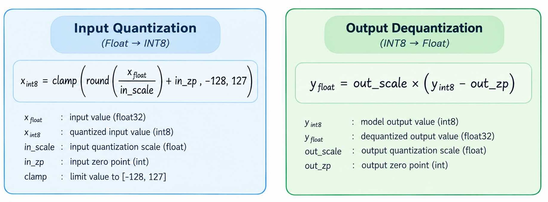
The full-INT8 TFLite model contains quantization parameters for its input and output tensors. The input quantization and output dequantization are performed in the application, so these values used in the app must match what the model expects.

After generating:

onnx2tf_normalized_full_int8/best_normalized_output_full_integer_quant.tflite

read the input and output scale and zero-point values from that TFLite model.

Read the values from the TFLite model

Save the following script as check_quantization.py in the directory containing the generated TFLite model:

import tensorflow as tf

MODEL = "onnx2tf_normalized_full_int8/best_normalized_output_full_integer_quant.tflite"

interpreter = tf.lite.Interpreter(model_path=MODEL)
interpreter.allocate_tensors()

input_details = interpreter.get_input_details()[0]
output_details = interpreter.get_output_details()[0]

input_q = input_details["quantization_parameters"]
output_q = output_details["quantization_parameters"]

in_scale = float(input_q["scales"][0])
in_zp = int(input_q["zero_points"][0])

out_scale = float(output_q["scales"][0])
out_zp = int(output_q["zero_points"][0])

print("in_scale =", in_scale)
print("in_zp    =", in_zp)
print("out_scale =", out_scale)
print("out_zp    =", out_zp)

Run:

python check_quantization.py

For example, the validated model reported values similar to:

in_scale = 0.003921568859368563
in_zp = -128
out_scale = 0.004194467328488827
out_zp = -128

Use the values printed for your generated model. Do not assume that the values from the example model will be correct for a retrained model.

Update sl2610-examples/object_detection

The Synaptics Astra SL2610-Series has a set of example applications at sl2610-examples, including an object_detection example based on YOLOv8.

The object-detection application includes the quantization parameters in the application code.

If using the image example, open:

sl2610-examples/object_detection/object_detection.py (or depending on the version: object_detection_video.py or run_cli.py)

Find the input quantization values in the preprocessing code:

in_scale = 0.003921568859368563
in_zp = -128

Replace them with the in_scale and in_zp values printed by check_quantization.py.

Then find the output dequantization values:

out_scale = 0.004194467328488827
out_zp = -128

Replace them with the out_scale and out_zp values printed by the script.

The application continues to perform quantization and dequantization exactly as before. Only the four parameters need to be updated so that they match the newly generated model.

The input values may remain the same when the same [0,1] preprocessing and INT8 conversion settings are used, but they should still be verified. The output quantization parameters are model-dependent and may change after retraining or recalibration, so they should always be checked for a newly converted model.

---

7. Convert TFLite to TOSA MLIR

MLIR (Multi-Level Intermediate Representation) is a compiler framework for representing and transforming programs and machine-learning models. TOSA (Tensor Operator Set Architecture) provides a standardized set of tensor operations within MLIR, giving the Torq compiler an intermediate representation that it can lower and compile for the NPU.

Convert the full INT8 TFLite model into TOSA MLIR:

tosa-converter-for-tflite \
  onnx2tf_normalized_full_int8/best_normalized_output_full_integer_quant.tflite \
  --text \
  -o normalized_full_integer.tosa.mlir

The result is normalized_full_integer.tosa.mlir.

---

8. Compile the Model for Torq

Compile the TOSA MLIR model:

torq-compile \
  normalized_full_integer.tosa.mlir \
  -o new.vmfb

The result is new.vmfb.

During compilation, the compiler may print a memory-planning warning such as Failed to swap in operand. This can be safely ignored if compilation completes successfully and the generated model produces accurate inference results. If the compiler crashes or fails to generate the VMFB, or if inference results are inaccurate, investigate the warning further.

For the validated workflow, compilation completed successfully with EXIT=0.

---

9. Run the Compiled VMFB

After compiling the model, switch to the target Synaptics Astra SL2610 or Coralboard and copy the new VMFB to the board.

For example, using ADB:

adb push new.vmfb /home/root/

The first test should be a simple runtime smoke test. The purpose of this test is only to confirm that the VMFB loads and executes successfully with the expected input shape and datatype. It is not intended to verify detection accuracy.

Create an all-zero INT8 input tensor with the model's expected input shape:

python3 -c 'import numpy as np; np.save("zero_input.npy", np.zeros((1,320,320,3), dtype=np.int8))'

Run the compiled VMFB:

torq-run-module \
  --module=new.vmfb \
  --function=main \
  --input=@zero_input.npy \
  --output=@output.npy

A successful execution should include EXEC @main.

At this point, we have confirmed that the compiled VMFB can be loaded and executed by the Torq runtime on the target board.

---

10. Testing the Model

The sl2610-examples repository provides an object detection example based on YOLOv8 that runs on the SL2610-series kits, including the Coralboard SL.

The example application handles the YOLO-specific preprocessing, quantization, NPU inference, and post-processing required to produce object detections.

Install the example dependencies

On the board, follow the sl2610-examples setup instructions in README.md.

Then install the object-detection dependencies:

cd object_detection
pip install -r requirements.txt

Run object detection with the new model

The application can take USB camera input and run inference using the Torq NPU.

Locate and update the application-side quantization parameters in_scale and out_scale in the application files as needed for your new custom model.

Pass the newly compiled VMFB with --model:

python3 object_detection_video.py   --model <your-model>.vmfb   --camera-device auto   --labels <your-labels>.json   --device torq

or depending on the version:

python3 run_cli.py   --model <your-model>.vmfb   --camera-device auto   --labels <your-labels>.json   --device torq

Replace:

• <your-model>.vmfb with the path to the VMFB generated in the previous steps.
• <your-labels>.json with the labels corresponding to the model.

For the custom model, make sure the labels and application-side quantization parameters match the model being used. The default model and labels provided by the example repository may correspond to a different YOLOv8 model.

To check available cameras:

v4l2-ctl --list-devices

You can then replace auto with a specific device such as /dev/video0 if needed.

Coralboard with OV5647 camera

For a Coralboard using the OV5647 MIPI CSI camera and MIPI DSI display, the example repository provides:

python3 object_detection_video.py   --camera-device /dev/video0   --camera-control-device /dev/v4l-subdev2   --display

The application performs the complete inference pipeline: Camera input -> YOLO preprocessing -> Quantization -> Torq NPU inference -> Dequantization / post-processing -> Object detections.

A successful test should produce detections with bounding boxes and confidence scores, confirming that the new VMFB works with the complete object-detection application.

For additional camera, video-file, RTSP, and display options, see the object_detection documentation in the sl2610-examples repository.

---

Putting It All Together

The complete workflow is Custom dataset -> Ultralytics training -> YOLOv8 best.pt -> Ultralytics ONNX export -> YOLOv8 ONNX -> normalize detection coordinates -> Normalized-output ONNX -> onnx2tf 2.6.8 with full INT8 quantization, representative calibration data, and the tf_converter backend -> Full INT8 TFLite -> tosa-converter-for-tflite -> TOSA MLIR -> torq-compile -> VMFB -> torq-run-module -> Torq inference.

For reproducibility:

• Keep training and export image sizes consistent.
• Use representative calibration images with the same preprocessing expected by the model.
• For the validated 320x320 model, normalize the first four output channels by 320.
• Use onnx2tf 2.6.8 and the tf_converter backend for the validated full-INT8 conversion.
• Record the Torq compiler version or source revision used to build the VMFB.
• Treat tensor shapes, output normalization, and other graph changes as model-specific.

Conclusion

Ultralytics provides a straightforward way to retrain YOLOv8, while the Torq conversion toolchain provides the path from a trained PyTorch model to an NPU-ready VMFB.

For the validated 320x320 model, the complete workflow successfully moved from a retrained .pt checkpoint through ONNX, full INT8 TFLite, TOSA MLIR, and finally a VMFB compiled with the current Torq toolchain. The resulting VMFB was validated against an existing compiled model and produced an exact output match.

This workflow provides a repeatable starting point for taking custom YOLOv8 object-detection models from training to deployment on the Synaptics Torq NPU.

Ultralytics and YOLOv8 are trademarks of Ultralytics Inc.; Ultralytics YOLO is distributed under the AGPL-3.0 license (a commercial license is also available from Ultralytics).