在 Synaptics Torq NPU 上部署自定义 YOLO 模型

在图像或摄像头画面中检测目标，是边缘 AI 中非常常见且实用的视觉应用场景，例如在工地检测安全帽以保障作业安全，或检测车辆以进行交通监控。预训练的目标检测模型通常无法检测你的应用所需的目标，因此在实际产品中，开发者需要重新训练模型。本文将介绍一个实用的工作流：重新训练目标检测模型，并将其转换为可在 Astra SL2610 系列处理器中的 Torq™ NPU 上运行的格式。

关于 YOLO 和 Ultralytics

YOLO（"You Only Look Once"）是一个流行的目标检测模型系列。它只需对图像进行一次处理即可检测出目标，因此足够高效，可以在许多平台上实时运行。YOLO 是单阶段检测器：图像依次经过卷积主干网络（backbone）、多尺度特征金字塔颈部（neck），以及在网格上预测边界框和类别的检测头（head）。YOLOv8 Nano（YOLOv8n） 是一个稳定、高效且被广泛部署的 YOLO 版本，本文示例即使用该模型。

Ultralytics 提供预训练模型和训练工具，帮助开发者根据自身需求重新训练模型。他们维护着 ultralytics Python 包，其中集成了 YOLOv8 及后续 YOLO 模型系列，以及训练、验证、预测和导出的完整工作流。这些模型底层基于 PyTorch——检查点就是标准的 .pt 文件——因此你可以在自定义数据集上进行微调，并导出为 ONNX、TFLite 等格式。与使用任何软件或工具一样，请务必查看 Ultralytics 的许可条款，确保其与你的项目兼容。

从训练到部署的工作流

经过验证的模型重训练与部署流程为：YOLOv8 training -> Model Export & Preprocessing -> Quantization -> Conversion to TOSA -> Compilation。

此处展示的转换步骤已在 320 x 320 的 YOLOv8 目标检测模型上验证。部分细节（尤其是输出归一化和张量形状）与具体模型相关，用于其他模型时需要相应调整。

---

前提条件

请在配备 GPU 的 Linux 开发系统上运行训练和转换工作流。

创建并激活 Python 虚拟环境：

python3 -m venv .venv
source .venv/bin/activate

安装 Ultralytics：

pip install -U ultralytics

验证安装：

yolo checks

Ultralytics 文档：

• Ultralytics Quickstart
• Ultralytics Train Mode
• Ultralytics Export Mode

转换流程还需要开发环境中具备以下工具：

• onnx2tf
• onnxsim
• tosa-converter-for-tflite
• torq-compile
• torq-run-module

经过验证的工作流使用的是 onnx2tf 2.6.8。

安装命令：

pip install onnx2tf==2.6.8
pip install onnxsim

Torq 编译器和 TOSA 转换工具请按照 Torq 官方文档进行安装：

• Torq Compiler Getting Started
• Torq Model Conversion

验证所需命令是否可用：

onnx2tf -V
which onnxsim
which tosa-converter-for-tflite
which torq-compile
which torq-run-module

---

1. 准备 YOLO 数据集

有大量资源可以帮助你生成带标注图像的自定义数据集，其中许多都支持导出为 Ultralytics 使用的 YOLO 兼容格式。

Ultralytics 使用数据集 YAML 文件来描述训练和验证数据。

典型的目标检测数据集结构如下：

dataset/
├── images/
│   ├── train/
│   └── val/
├── labels/
│   ├── train/
│   └── val/
└── data.yaml

每张图像都有一个对应的 YOLO 格式标签文件。

一个简单的 data.yaml 示例如下：

path: /path/to/dataset
train: images/train
val: images/val

names:
  0: object

请根据你的项目更新数据集路径和类别名称。

---

2. 使用 Ultralytics 重新训练 YOLOv8

从预训练的 YOLOv8n 检查点开始，在自定义数据集上进行微调。

yolo detect train \
  model=yolov8n.pt \
  data=data.yaml \
  epochs=100 \
  imgsz=320

在经过验证的 Torq 工作流中，模型输入分辨率为 320 x 320。

训练会在 Ultralytics 的运行目录下生成检查点。通常用于部署的检查点是 best.pt。

在进入部署之前，先验证训练好的模型：

yolo detect val model=best.pt data=data.yaml

你也可以在具有代表性的图像上运行预测：

yolo detect predict model=best.pt source=/path/to/test/images

当 .pt 模型表现符合预期后，即可进行部署转换。

---

3. 将 PyTorch 模型导出为 ONNX

将训练好的模型导出为 ONNX。ONNX 格式在按需修改模型方面具有最大的灵活性。

yolo export \
  model=best.pt \
  format=onnx \
  imgsz=320

导出结果为 best.onnx。

---

4. 归一化检测输出

对于经过验证的 320x320 模型，ONNX 输出张量为 output0: [1, 5, 2100]。

各维度含义如下：

• 1 - 批大小（batch size）
• 5 - 每个候选预测的五个值：四个边界框坐标和一个置信度值
• 2100 - 模型生成的候选预测数量

2100 这一维度并不表示模型检测到了 2100 个目标。模型生成的是候选预测，这些候选预测随后经过筛选和后处理，得到最终的检测结果。因此，一张图像的检测结果可能是零个、一个或多个目标。

对于该模型，前四个输出通道包含边界框坐标，第五个通道包含置信度值。边界框坐标需要按照 320x320 的输入分辨率进行归一化：boxes = output0[:, 0:4, :] / 320，confidence = output0[:, 4:5, :]，以及 normalized_output = concat(boxes, confidence, axis=1)。

数值 320 即模型的输入分辨率 [1, 3, 320, 320]。

它是输出坐标的归一化系数，而不是 INT8 量化参数。

应用归一化

归一化直接在 ONNX 图中实现。

下面的脚本会：

1. 加载导出的 ONNX 模型。
2. 提取前四个输出通道。
3. 将边界框坐标除以 320。
4. 原样提取置信度通道。
5. 将归一化后的边界框与置信度值拼接。
6. 用归一化后的输出替换原始图输出。
7. 保存生成的 ONNX 模型。

将以下内容保存为 normalize_output.py，并放在与 best.onnx 相同的目录中：

import onnx
from onnx import helper, TensorProto, numpy_helper
import numpy as np

SRC = "best.onnx"
DST = "best_normalized_output.onnx"

m = onnx.load(SRC)

starts_box = numpy_helper.from_array(
    np.array([0], dtype=np.int64),
    name="norm_starts_box",
)
ends_box = numpy_helper.from_array(
    np.array([4], dtype=np.int64),
    name="norm_ends_box",
)
axes = numpy_helper.from_array(
    np.array([1], dtype=np.int64),
    name="norm_axes",
)
steps = numpy_helper.from_array(
    np.array([1], dtype=np.int64),
    name="norm_steps",
)

starts_conf = numpy_helper.from_array(
    np.array([4], dtype=np.int64),
    name="norm_starts_conf",
)
ends_conf = numpy_helper.from_array(
    np.array([5], dtype=np.int64),
    name="norm_ends_conf",
)

scale320 = numpy_helper.from_array(
    np.array([320.0], dtype=np.float32),
    name="norm_scale_320",
)

m.graph.initializer.extend([
    starts_box,
    ends_box,
    axes,
    steps,
    starts_conf,
    ends_conf,
    scale320,
])

slice_box = helper.make_node(
    "Slice",
    inputs=[
        "output0",
        "norm_starts_box",
        "norm_ends_box",
        "norm_axes",
        "norm_steps",
    ],
    outputs=["normalized_boxes_input"],
    name="NormalizeOutput_SliceBoxes",
)

div_box = helper.make_node(
    "Div",
    inputs=["normalized_boxes_input", "norm_scale_320"],
    outputs=["normalized_boxes"],
    name="NormalizeOutput_Div320",
)

slice_conf = helper.make_node(
    "Slice",
    inputs=[
        "output0",
        "norm_starts_conf",
        "norm_ends_conf",
        "norm_axes",
        "norm_steps",
    ],
    outputs=["normalized_confidence"],
    name="NormalizeOutput_SliceConfidence",
)

concat = helper.make_node(
    "Concat",
    inputs=["normalized_boxes", "normalized_confidence"],
    outputs=["normalized_output"],
    axis=1,
    name="NormalizeOutput_Concat",
)

m.graph.node.extend([
    slice_box,
    div_box,
    slice_conf,
    concat,
])

del m.graph.output[:]

m.graph.output.append(
    helper.make_tensor_value_info(
        "normalized_output",
        TensorProto.FLOAT,
        [1, 5, 2100],
    )
)

onnx.checker.check_model(m)
onnx.save(m, DST)

print("Created:", DST)

运行：

python normalize_output.py

预期输出 Created: best_normalized_output.onnx

生成的模型为 best_normalized_output.onnx

输出形状仍为 [1, 5, 2100]

此归一化步骤与具体模型相关。如果其他模型的输出表示或输入分辨率不同，则必须针对该模型确定相应的输出通道和归一化系数。

---

5. 准备用于量化的代表性校准数据

完整的 INT8 量化需要具有代表性的校准样本。经过验证的转换使用了 300 张代表性图像。

模型的输入图像需要满足以下格式：

• RGB
• 320 x 320 letterbox
• NHWC
• float32
• 取值范围 [0, 1]

使用以下脚本创建图像集：

import cv2
import numpy as np
from pathlib import Path

IMAGE_DIR = Path("calibration_images")
OUTPUT = "calibration_video_300_nhwc_float32.npy"
SIZE = 320
MAX_IMAGES = 300

samples = []

paths = sorted(
    list(IMAGE_DIR.glob("*.jpg"))
    + list(IMAGE_DIR.glob("*.jpeg"))
    + list(IMAGE_DIR.glob("*.png"))
)[:MAX_IMAGES]

for path in paths:
    image = cv2.imread(str(path))
    if image is None:
        continue

    image = cv2.cvtColor(image, cv2.COLOR_BGR2RGB)

    height, width = image.shape[:2]
    scale = min(SIZE / width, SIZE / height)

    new_width = int(round(width * scale))
    new_height = int(round(height * scale))

    resized = cv2.resize(image, (new_width, new_height))
    padded = np.full((SIZE, SIZE, 3), 114, dtype=np.uint8)

    top = (SIZE - new_height) // 2
    left = (SIZE - new_width) // 2
    padded[top:top + new_height, left:left + new_width] = resized

    samples.append(padded.astype(np.float32) / 255.0)

if not samples:
    raise RuntimeError("No calibration images were processed.")

calibration = np.stack(samples).astype(np.float32)
np.save(OUTPUT, calibration)

print("Created:", OUTPUT)
print("Shape:", calibration.shape)
print("Dtype:", calibration.dtype)
print("Range:", float(calibration.min()), float(calibration.max()))

验证结果：

python -c 'import numpy as np; a=np.load("calibration_video_300_nhwc_float32.npy"); print("shape:",a.shape); print("dtype:",a.dtype); print("range:",float(a.min()),float(a.max()))'

预期输出：shape: (300, 320, 320, 3)、dtype: float32 以及 range: 0.0 ... 1.0。

校准数据已归一化到 [0,1]，因此在转换过程中不要再除以 255。

---

6. 将 ONNX 转换为全 INT8 TFLite

ONNX 模型使用 NCHW 图像格式，即 [1, 3, 320, 320]。

在本示例中，我们将其转换为使用 NHWC 图像格式（[1, 320, 320, 3]）的 TFLite。

之所以进行这一转换，是因为下文引用的示例应用需要该格式；不过根据你的应用软件，这一步是可选的。

在经过验证的工作流中，使用 onnx2tf 工具并选用 tf_converter 后端。

onnx2tf \
  -i best_normalized_output.onnx \
  -o onnx2tf_normalized_full_int8 \
  -oiqt \
  -iqd int8 \
  -oqd int8 \
  --tflite_backend tf_converter \
  -cind images calibration_video_300_nhwc_float32.npy \
  "[[[[0.0,0.0,0.0]]]]" \
  "[[[[1.0,1.0,1.0]]]]"

onnx2tf 各选项的作用

• -i best_normalized_output.onnx - 指定要转换的归一化 ONNX 模型。
• -o onnx2tf_normalized_full_int8 - 指定生成的 TFLite 文件的输出目录。
• -oiqt - 为 TFLite 模型启用整数量化。
• -iqd int8 - 指定模型输入为 INT8。
• -oqd int8 - 指定模型输出为 INT8。
• --tflite_backend tf_converter - 选择 TensorFlow 转换器后端。经过验证的工作流必须使用该后端，因为另一个 flatbuffer_direct 后端生成的 TFLite 表示在后续 TFLite 到 TOSA 的转换中会失败。
• -cind images - 指定校准数据所对应的 ONNX 输入张量名称（images）。
• calibration_video_300_nhwc_float32.npy - 提供 INT8 校准时使用的代表性校准样本。
• [[[[0.0,0.0,0.0]]]] - 指定三个图像通道的输入范围下限。
• [[[[1.0,1.0,1.0]]]] - 指定三个图像通道的输入范围上限。

这些选项共同生成一个全 INT8 的 TFLite 模型。在此转换过程中，onnx2tf 会使用代表性校准数据来确定量化参数。

输出文件为 onnx2tf_normalized_full_int8/best_normalized_output_full_integer_quant.tflite。

预期接口：

• INPUT: [1, 320, 320, 3] (int8)
• OUTPUT: [1, 5, 2100] (int8)

tf_converter 后端对这一经过验证的工作流非常重要。使用默认的 flatbuffer_direct 后端进行测试时，由于量化缩放（scale）约束，生成的表示在后续 TFLite 到 TOSA 的转换中失败了。

---

更新应用中的量化参数

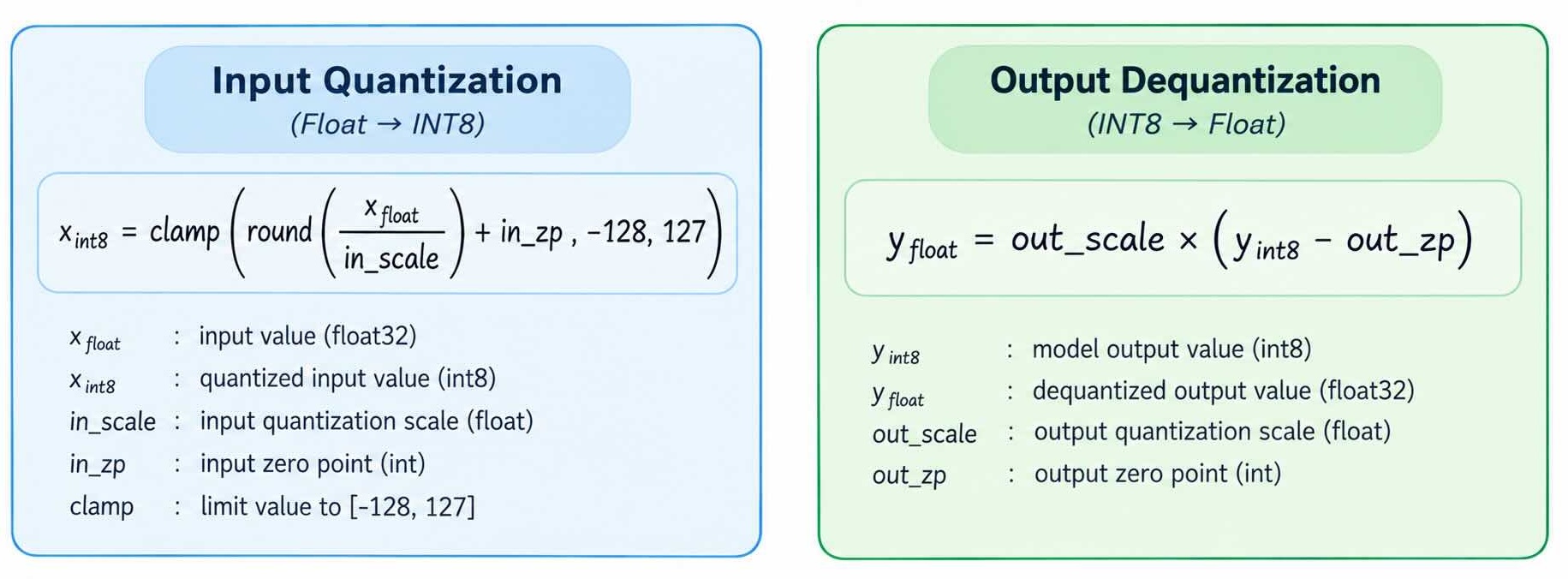
全 INT8 TFLite 模型包含其输入和输出张量的量化参数。输入量化和输出反量化在应用中完成，因此应用中使用的这些数值必须与模型的预期一致。

生成以下文件后：

onnx2tf_normalized_full_int8/best_normalized_output_full_integer_quant.tflite

从该 TFLite 模型中读取输入和输出的 scale 与 zero-point 值。

从 TFLite 模型中读取数值

将以下脚本保存为 check_quantization.py，并放在包含所生成 TFLite 模型的目录中：

import tensorflow as tf

MODEL = "onnx2tf_normalized_full_int8/best_normalized_output_full_integer_quant.tflite"

interpreter = tf.lite.Interpreter(model_path=MODEL)
interpreter.allocate_tensors()

input_details = interpreter.get_input_details()[0]
output_details = interpreter.get_output_details()[0]

input_q = input_details["quantization_parameters"]
output_q = output_details["quantization_parameters"]

in_scale = float(input_q["scales"][0])
in_zp = int(input_q["zero_points"][0])

out_scale = float(output_q["scales"][0])
out_zp = int(output_q["zero_points"][0])

print("in_scale =", in_scale)
print("in_zp    =", in_zp)
print("out_scale =", out_scale)
print("out_zp    =", out_zp)

运行：

python check_quantization.py

例如，经过验证的模型输出的数值类似于：

in_scale = 0.003921568859368563
in_zp = -128
out_scale = 0.004194467328488827
out_zp = -128

请使用你所生成模型实际打印出的数值。不要假定示例模型的数值适用于重新训练后的模型。

更新 sl2610-examples/object_detection

Synaptics Astra SL2610 系列提供了一组示例应用 sl2610-examples，其中包括一个基于 YOLOv8 的 object_detection 示例。

目标检测应用在应用代码中包含了量化参数。

如果使用图像示例，请打开：

sl2610-examples/object_detection/object_detection.py（根据版本不同，也可能是 object_detection_video.py 或 run_cli.py）

在预处理代码中找到输入量化值：

in_scale = 0.003921568859368563
in_zp = -128

将它们替换为 check_quantization.py 打印出的 in_scale 和 in_zp 值。

然后找到输出反量化值：

out_scale = 0.004194467328488827
out_zp = -128

将它们替换为脚本打印出的 out_scale 和 out_zp 值。

应用仍会与之前完全相同地执行量化和反量化，只需更新这四个参数，使其与新生成的模型相匹配。

当使用相同的 [0,1] 预处理和 INT8 转换设置时，输入值可能保持不变，但仍应进行核实。输出量化参数与模型相关，在重新训练或重新校准后可能发生变化，因此对于新转换的模型，务必检查这些参数。

---

7. 将 TFLite 转换为 TOSA MLIR

MLIR（Multi-Level Intermediate Representation，多级中间表示）是一个用于表示和转换程序及机器学习模型的编译器框架。TOSA（Tensor Operator Set Architecture，张量算子集架构）在 MLIR 中提供了一组标准化的张量运算，为 Torq 编译器提供一种可以降低（lower）并编译到 NPU 的中间表示。

将全 INT8 TFLite 模型转换为 TOSA MLIR：

tosa-converter-for-tflite \
  onnx2tf_normalized_full_int8/best_normalized_output_full_integer_quant.tflite \
  --text \
  -o normalized_full_integer.tosa.mlir

转换结果为 normalized_full_integer.tosa.mlir。

---

8. 为 Torq 编译模型

编译 TOSA MLIR 模型：

torq-compile \
  normalized_full_integer.tosa.mlir \
  -o new.vmfb

编译结果为 new.vmfb。

编译期间，编译器可能会打印内存规划相关的警告，例如 Failed to swap in operand。如果编译成功完成，且生成的模型能给出准确的推理结果，则可以放心忽略该警告。如果编译器崩溃、无法生成 VMFB，或推理结果不准确，则需要进一步排查该警告。

在经过验证的工作流中，编译成功完成，返回 EXIT=0。

---

9. 运行编译后的 VMFB

模型编译完成后，切换到目标 Synaptics Astra SL2610 或 Coralboard，并将新的 VMFB 复制到开发板上。

例如，使用 ADB：

adb push new.vmfb /home/root/

第一个测试应当是简单的运行时冒烟测试（smoke test）。该测试的目的仅是确认 VMFB 能以预期的输入形状和数据类型成功加载并执行，并不用于验证检测精度。

按照模型预期的输入形状创建一个全零的 INT8 输入张量：

python3 -c 'import numpy as np; np.save("zero_input.npy", np.zeros((1,320,320,3), dtype=np.int8))'

运行编译后的 VMFB：

torq-run-module \
  --module=new.vmfb \
  --function=main \
  --input=@zero_input.npy \
  --output=@output.npy

成功执行时，输出中应包含 EXEC @main。

至此，我们已确认编译后的 VMFB 可以在目标开发板上由 Torq 运行时加载并执行。

---

10. 测试模型

sl2610-examples 仓库提供了一个基于 YOLOv8 的目标检测示例，可在包括 Coralboard SL 在内的 SL2610 系列套件上运行。

该示例应用负责完成生成目标检测结果所需的 YOLO 专用预处理、量化、NPU 推理和后处理。

安装示例依赖

在开发板上，按照 README.md 中的 sl2610-examples 设置说明进行操作。

然后安装目标检测所需的依赖：

cd object_detection
pip install -r requirements.txt

使用新模型运行目标检测

该应用可以接收 USB 摄像头输入，并使用 Torq NPU 运行推理。

根据你的新自定义模型，在应用文件中找到并更新应用侧的量化参数 in_scale 和 out_scale。

通过 --model 传入新编译的 VMFB：

python3 object_detection_video.py   --model <your-model>.vmfb   --camera-device auto   --labels <your-labels>.json   --device torq

或根据版本不同：

python3 run_cli.py   --model <your-model>.vmfb   --camera-device auto   --labels <your-labels>.json   --device torq

替换：

• <your-model>.vmfb 为前面步骤中生成的 VMFB 路径。
• <your-labels>.json 为与模型对应的标签文件。

对于自定义模型，请确保标签和应用侧量化参数与所使用的模型相匹配。示例仓库中提供的默认模型和标签可能对应的是另一个 YOLOv8 模型。

查看可用的摄像头：

v4l2-ctl --list-devices

如有需要，可以将 auto 替换为特定设备，例如 /dev/video0。

使用 OV5647 摄像头的 Coralboard

对于使用 OV5647 MIPI CSI 摄像头和 MIPI DSI 显示屏的 Coralboard，示例仓库提供了以下命令：

python3 object_detection_video.py   --camera-device /dev/video0   --camera-control-device /dev/v4l-subdev2   --display

该应用会执行完整的推理流水线：Camera input -> YOLO preprocessing -> Quantization -> Torq NPU inference -> Dequantization / post-processing -> Object detections。

测试成功时，应能输出带有边界框和置信度分数的检测结果，从而确认新的 VMFB 能在完整的目标检测应用中正常工作。

有关更多摄像头、视频文件、RTSP 和显示选项，请参阅 sl2610-examples 仓库中的 object_detection 文档。

---

总结整个流程

完整的工作流为：Custom dataset -> Ultralytics training -> YOLOv8 best.pt -> Ultralytics ONNX export -> YOLOv8 ONNX -> normalize detection coordinates -> Normalized-output ONNX -> onnx2tf 2.6.8 with full INT8 quantization, representative calibration data, and the tf_converter backend -> Full INT8 TFLite -> tosa-converter-for-tflite -> TOSA MLIR -> torq-compile -> VMFB -> torq-run-module -> Torq inference。

为确保可复现性：

• 保持训练和导出时的图像尺寸一致。
• 使用与模型预期预处理方式相同的代表性校准图像。
• 对于经过验证的 320x320 模型，将前四个输出通道除以 320 进行归一化。
• 在经过验证的全 INT8 转换中，使用 onnx2tf 2.6.8 和 tf_converter 后端。
• 记录构建 VMFB 所用的 Torq 编译器版本或源码修订版本。
• 将张量形状、输出归一化及其他图修改视为与具体模型相关。

结论

Ultralytics 提供了重新训练 YOLOv8 的便捷方式，而 Torq 转换工具链则提供了从训练好的 PyTorch 模型到可在 NPU 上运行的 VMFB 的完整路径。

对于经过验证的 320x320 模型，完整工作流成功地从重新训练的 .pt 检查点出发，依次经过 ONNX、全 INT8 TFLite、TOSA MLIR，最终生成了由当前 Torq 工具链编译的 VMFB。生成的 VMFB 已与现有的编译模型进行对比验证，输出完全一致。

该工作流为将自定义 YOLOv8 目标检测模型从训练推进到 Synaptics Torq NPU 上的部署，提供了一个可重复使用的起点。

Ultralytics 和 YOLOv8 是 Ultralytics Inc. 的商标；Ultralytics YOLO 以 AGPL-3.0 许可证分发（也可从 Ultralytics 获取商业许可证）。